↗ OpenReview ↗ NeurIPS Proc. ↗ Chat
TL;DR#
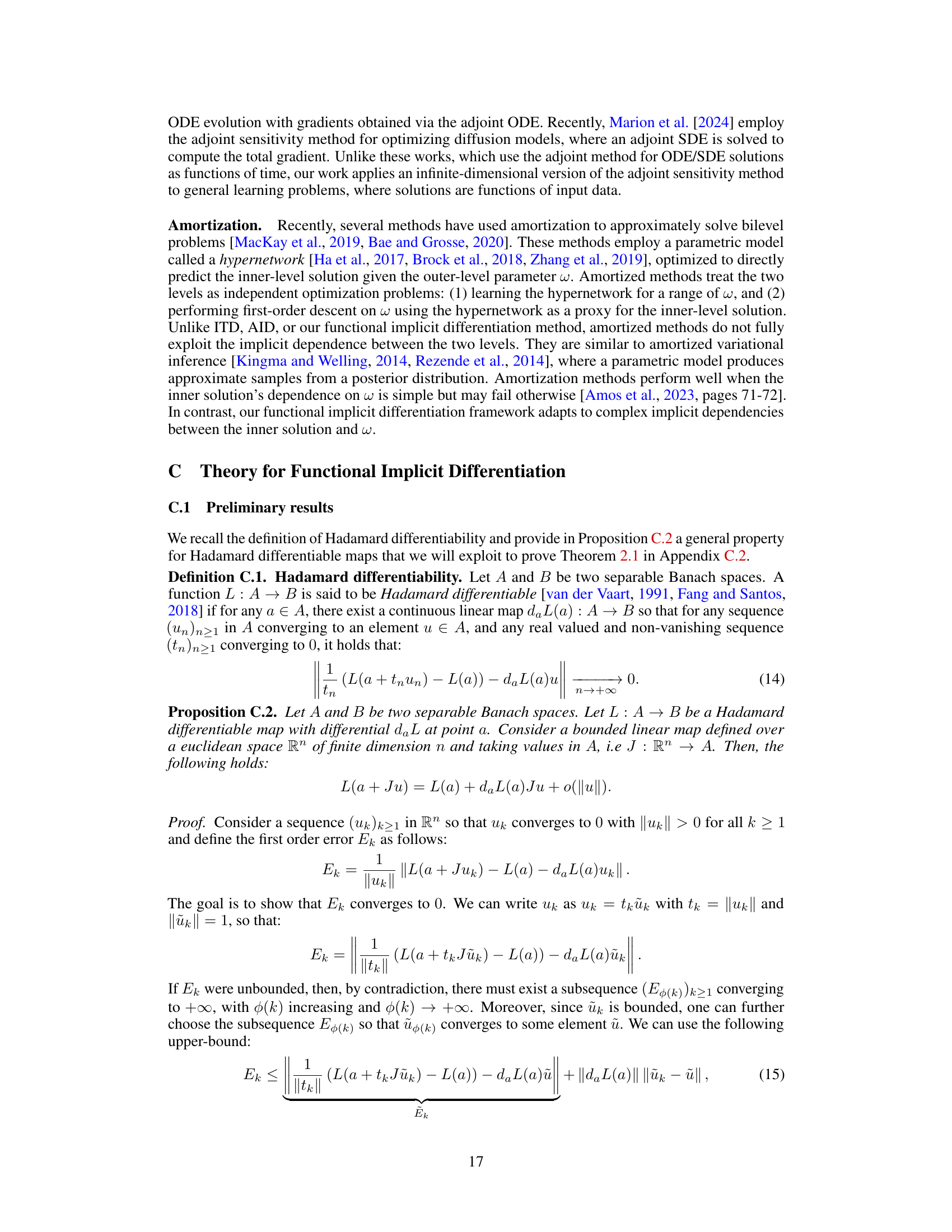
Many machine learning problems can be formulated as bilevel optimization problems, where an outer-level objective is optimized subject to an inner-level optimization problem. Existing methods often struggle with issues related to non-convexity, multiple inner-level solutions, and sensitivity to parameterization, especially when using neural networks.
This research introduces a novel functional approach to address these issues. Instead of optimizing over the parameters of the inner-level function, they propose to optimize directly over the function space, ensuring a unique solution. This approach allows the use of over-parameterized models like neural networks without sacrificing theoretical guarantees. They propose scalable algorithms for this functional perspective and demonstrate the benefits of their approach on instrumental regression and reinforcement learning tasks.
Key Takeaways#
Why does it matter?#
This paper is crucial for researchers working on bilevel optimization and machine learning. It offers a novel functional perspective that resolves ambiguity issues in existing methods, providing scalable algorithms with strong convergence guarantees. The proposed framework opens up new avenues for research in various applications, such as instrumental regression and reinforcement learning. Its impact lies in improving the stability, efficiency and effectiveness of bilevel optimization algorithms.
Visual Insights#

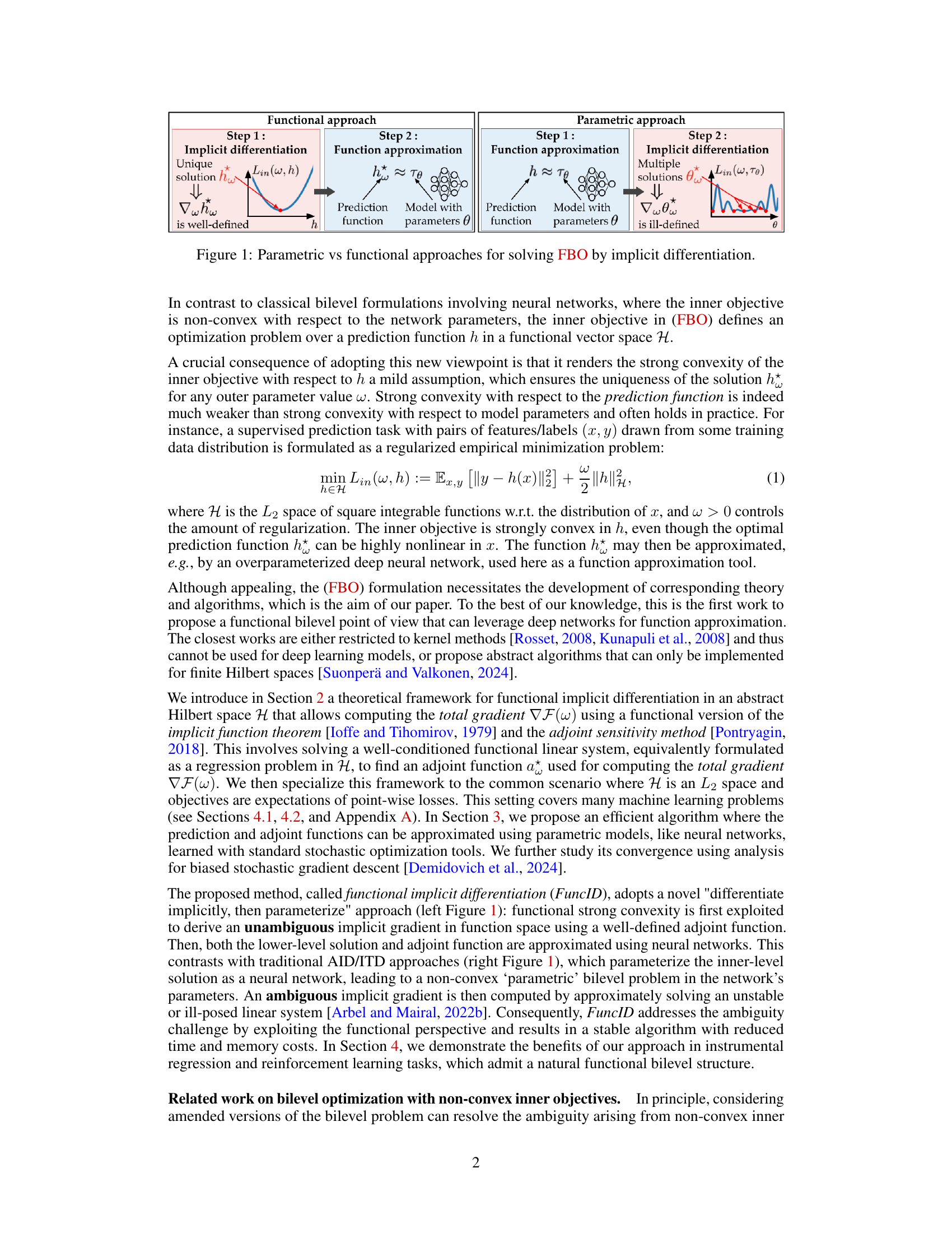
This figure compares the parametric and functional approaches to bilevel optimization, focusing on the implicit differentiation step. The functional approach, which the paper proposes, first performs implicit differentiation in a function space, resulting in a well-defined solution, and then approximates this solution with a parameterized model. This contrasts with the parametric approach, where a parameterized model is used first, and implicit differentiation is then performed in the parameter space. The parametric approach often leads to multiple solutions and an ill-defined implicit gradient due to the non-convexity of the inner objective in the parameter space.

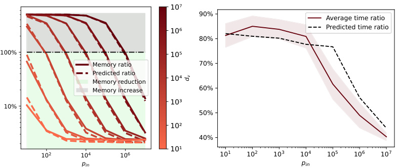
This table compares the computational cost (time and memory) of using AID vs FuncID for total gradient estimation in bilevel optimization. It breaks down the costs into components related to prediction and adjoint model evaluations, inner objective computations, and overheads for Hessian-vector products and gradient calculations. The table highlights the potential memory savings of FuncID over AID, particularly for deep networks, because FuncID does not require the computationally expensive computation of Hessian-vector products for the prediction network.
In-depth insights#
FuncID Algorithm#
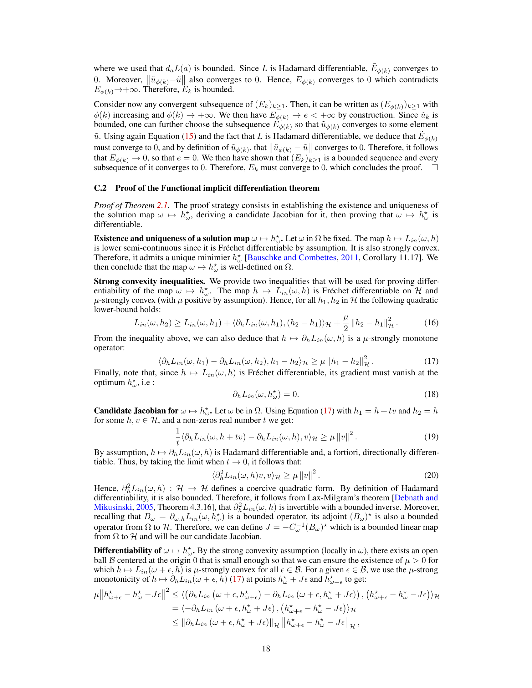
The FuncID algorithm, a novel approach to functional bilevel optimization, offers a compelling alternative to existing methods by directly tackling the challenges posed by non-convex inner objectives. FuncID leverages the strong convexity of the inner problem in function space, circumventing the ambiguities inherent in parameter-based approaches. This functional perspective enables the use of over-parameterized neural networks for function approximation, as the strong convexity assumption is placed on the function itself, not its parameters, a far weaker condition. The algorithm proceeds by first implicitly differentiating to find an adjoint function. This is computationally efficient and robust because it involves solving a well-conditioned linear system, unlike methods that require computationally expensive Hessian-vector products. Then, the prediction and adjoint functions are parameterized and learned using stochastic gradient descent, creating a practical and efficient algorithm. FuncID’s theoretical guarantees support its convergence to stationary points, addressing issues of ambiguity commonly encountered in bilevel optimization with neural networks. Overall, FuncID presents a unique blend of theoretical rigor and practical scalability, potentially opening up new avenues for applying bilevel optimization to complex machine learning problems.
Bilevel Optimization#
Bilevel optimization is a powerful technique for tackling hierarchical optimization problems, where the optimization of an outer-level objective is contingent on the solution of an inner-level problem. This nested structure is particularly relevant in machine learning, where it finds applications in various scenarios, including hyperparameter optimization, meta-learning, and domain adaptation. The core challenge in bilevel optimization lies in efficiently computing the gradients of the outer objective, which necessitates careful consideration of the inner problem’s solution and its sensitivity to the outer-level parameters. Methods like iterative differentiation and implicit differentiation have been proposed to address this challenge, but they often suffer from limitations, such as requiring strong convexity assumptions or being computationally expensive. Recent advancements, such as the functional approach discussed in the paper, aim to overcome these limitations by offering improved scalability and flexibility. The functional perspective provides a fresh look at this challenging problem and has the potential to unlock even more practical applications of bilevel optimization within the machine learning domain.
Functional Approach#
A functional approach to bilevel optimization offers a compelling alternative to traditional parametric methods, especially when dealing with non-convex inner problems. Instead of optimizing over a finite-dimensional parameter space, it directly tackles the optimization problem over a function space. This shift in perspective mitigates issues related to multiple inner solutions and ambiguous gradients, which often plague parametric methods when employing flexible models like neural networks. The functional approach leverages the inherent strong convexity of the inner objective in the function space to compute a well-defined total gradient through functional implicit differentiation, providing a more stable and efficient algorithm. This approach’s strength lies in its ability to naturally handle over-parameterized models and bypass the need for restrictive assumptions on strong convexity often required by parametric approaches. The resulting algorithms are scalable and efficient, as demonstrated by applications in instrumental regression and reinforcement learning.
Empirical Results#
An ‘Empirical Results’ section in a research paper would typically present the findings of experiments conducted to validate the paper’s claims. A strong section would begin by clearly stating the experimental setup, including datasets used, evaluation metrics, and any preprocessing steps. Specific details about the implementation of algorithms, such as hyperparameters and training procedures, should also be provided to ensure reproducibility. The presentation of results would then follow, ideally using visualizations (graphs, tables, etc.) to clearly communicate key findings. Statistical significance should be rigorously addressed, with error bars or p-values reported to indicate the confidence level of observed results. Furthermore, the section should discuss the obtained results in relation to the paper’s hypotheses, explaining any discrepancies and providing potential reasons. A thoughtful analysis should compare the performance of the proposed methods against relevant baselines and clearly state the relative strengths and weaknesses of each approach. Finally, the section should conclude with a concise summary of the main findings and their implications for the field.
Future Research#
The paper’s conclusion highlights several promising avenues for future research. Extending the functional framework beyond L2 spaces to encompass other function spaces, such as Reproducing Kernel Hilbert Spaces (RKHS) or Sobolev spaces, is a key area. This would broaden applicability and potentially reveal advantages for specific machine learning problems. Another important direction is handling non-smooth objectives or constrained optimization problems. Building upon existing work in non-smooth implicit differentiation could lead to significant advancements, especially in scenarios with complex constraints that are common in real-world applications. Finally, developing more efficient algorithms and exploring more sophisticated optimization techniques would improve the scalability and applicability of the functional bilevel optimization framework to a wider range of large-scale machine learning problems. Investigating the impact of different approximation methods on the overall accuracy and efficiency is another important aspect to be investigated.
More visual insights#
More on figures

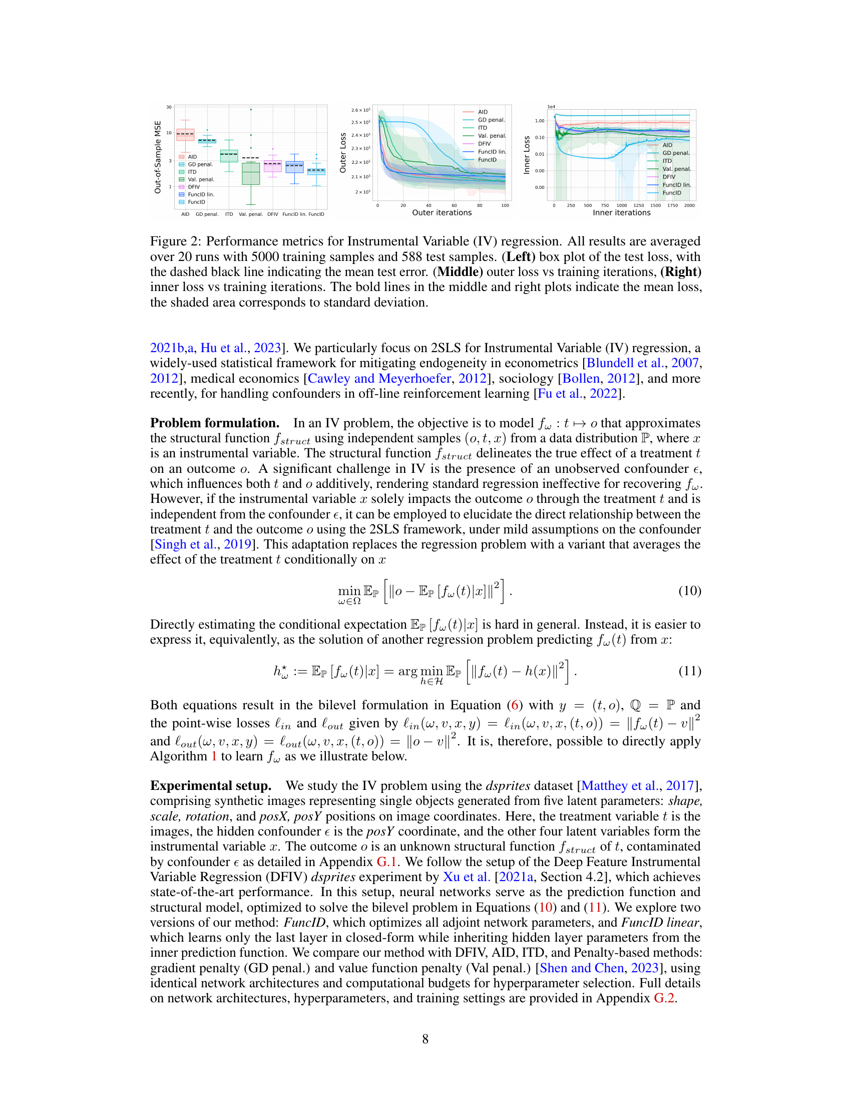
This figure compares different bilevel optimization methods on an instrumental variable regression task using the dsprites dataset. The left panel shows a box plot of the out-of-sample mean squared error (MSE) for each method, highlighting the performance of FuncID. The middle and right panels display the outer and inner losses, respectively, plotted against the number of outer and inner iterations. These plots reveal the convergence behavior of the algorithms, illustrating how FuncID achieves lower losses compared to other methods.
This figure compares the performance of several bilevel optimization methods on an instrumental variable regression task. The left panel shows a box plot of the out-of-sample mean squared error (MSE) for each method, indicating FuncID’s superior performance. The middle and right panels display the outer and inner losses, respectively, over training iterations. The plots show that FuncID converges faster and achieves lower losses than other methods.
This figure compares the performance of different bilevel optimization methods for instrumental variable regression. Three plots show the out-of-sample mean squared error (MSE), outer loss, and inner loss over training iterations. The left plot shows box plots of the test MSE, while the middle and right plots show the outer and inner losses with mean and standard deviation for each method. The results highlight the superior performance of the proposed FuncID method compared to other baselines.
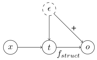
This figure is a causal graph showing the relationship between the treatment variable (t), outcome variable (o), instrumental variable (x), and unobserved confounder (e) in an instrumental variable regression setting. The arrows indicate the causal direction. The treatment variable is directly influenced by the unobserved confounder and the instrumental variable. The outcome is influenced by both the treatment variable and the unobserved confounder. The instrumental variable only influences the outcome through the treatment variable. This graph visually represents the causal structure used in the 2SLS experiment described in section 4.1.

This figure compares the performance of different bilevel optimization methods on an instrumental variable regression task. The left panel shows a box plot of the out-of-sample mean squared error (MSE) for each method, providing a summary of the model’s prediction accuracy. The middle and right panels show the evolution of the outer and inner losses, respectively, over training iterations, allowing for a comparison of convergence speed and stability.
This figure compares the performance of different bilevel optimization methods on the instrumental variable regression task. The left panel shows a box plot of the out-of-sample mean squared error (MSE) for each method, highlighting the test performance. The central and right panels present the evolution of the outer and inner losses during the training iterations, respectively, allowing for a more detailed analysis of convergence behavior. Shaded areas represent standard deviations, providing an indication of uncertainty in the results.
This figure compares the performance of various bilevel optimization methods on an instrumental variable regression task. The left panel shows a box plot summarizing the out-of-sample mean squared error (MSE) achieved by each method on a held-out test set. The middle and right panels display the training curves of the outer and inner objectives, respectively, showing how these losses evolve as the optimization progresses. The results indicate that the proposed FuncID method outperforms alternative approaches in terms of out-of-sample MSE.
More on tables

This table compares the computational cost (time and memory) of using AID and FuncID methods for a single total gradient estimation. It breaks down the cost into the time for evaluating the prediction and adjoint models, the time for inner objective evaluation, and overheads for Hessian-vector products and gradients. The memory cost is analyzed in terms of the cost of storing intermediate outputs, Hessian-vector products, and model parameters.

This table compares the computational cost (time and memory) of using AID vs FuncID for estimating the total gradient in bilevel optimization. It breaks down the costs into components related to model evaluation, inner-objective computations and Hessian-vector products. The table shows that FuncID generally has a lower computational cost, particularly in terms of memory, especially when the prediction model is a large neural network.
Full paper#
