↗ OpenReview ↗ NeurIPS Proc. ↗ Chat
TL;DR#
Reinforcement learning (RL) faces challenges like non-stationary environments, plasticity loss (where the model loses the capacity to learn new things), and the need for exploration (to prevent getting stuck in local optima). These issues limit RL’s performance and application. Existing solutions often rely on manual adjustments, limiting adaptability and scalability.
This paper introduces OPEN, an algorithm that meta-learns an update rule that addresses these three challenges. OPEN uses a flexible parameterization informed by existing techniques to boost exploration and handle non-stationarity and plasticity loss. Experiments show that OPEN matches or surpasses the performance of standard optimizers, particularly demonstrating strong generalization across various environments and agent structures.
Key Takeaways#
Why does it matter?#
This paper is important because it addresses critical challenges in reinforcement learning (RL) – non-stationarity, plasticity loss, and exploration – by introducing a novel meta-learning approach. The OPEN algorithm demonstrates significant performance improvements over traditional optimizers and learned optimizers, opening exciting avenues for future research in improving RL algorithm efficiency and generalization. It also provides valuable insights into how learned optimization can be designed to address specific RL difficulties and contributes valuable tools and benchmarks for future RL research.
Visual Insights#
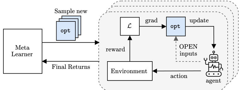
This figure illustrates the OPEN algorithm’s training process. Multiple RL agents are trained concurrently. Each agent uses a learned optimizer, sampled from a meta-learner, to update its parameters. The optimizers receive gradients, momentum, and additional handcrafted features as input (these features are detailed in Section 5.3 of the paper). The final return of each agent is then fed back to the meta-learner, allowing it to improve the learned optimizer over time. This process repeats, evolving the learned optimizer’s ability to improve the RL agent’s performance.
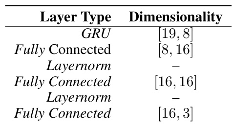
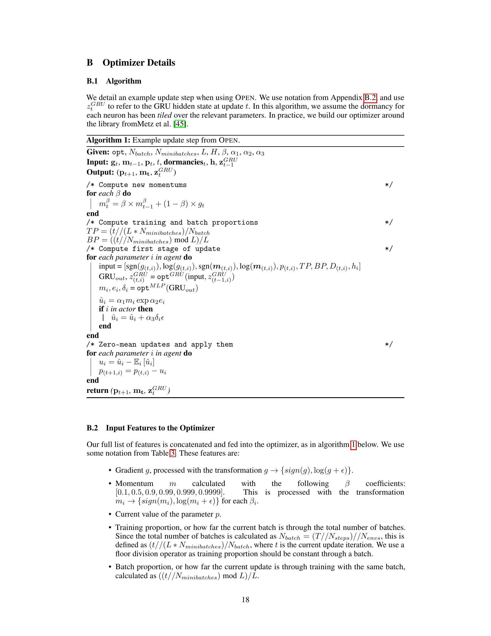
This table shows the layer types and their dimensionalities for the OPEN optimizer used in the single-task and gridworld experiments. The optimizer consists of a GRU followed by multiple fully connected layers with LayerNorm for stability. The dimensionalities specify the number of input and output units for each layer. This architectural configuration is crucial for the optimizer’s ability to process various inputs and generate appropriate updates.
In-depth insights#
Learned Optimizers for RL#
The application of learned optimizers to reinforcement learning (RL) presents a compelling avenue for enhancing the efficiency and effectiveness of RL algorithms. Traditional optimizers, such as Adam and RMSprop, often struggle with the inherent non-stationarity and plasticity challenges of RL. Learned optimizers offer a potential solution by adapting their update rules to the specific characteristics of the RL problem, potentially leading to faster convergence and improved generalization. Meta-learning techniques are particularly relevant for training learned optimizers, allowing them to learn effective update rules from experience across diverse environments. However, the success of learned optimizers in RL is critically dependent on careful design choices, including appropriate parameterizations, input features and training strategies. Challenges remain in ensuring robust generalization across different RL tasks and environments, and further research is needed to explore the full potential of learned optimizers in addressing the complexities of real-world RL applications.
OPEN Algorithm Details#
The heading ‘OPEN Algorithm Details’ suggests a section dedicated to explaining the inner workings of the OPEN algorithm, likely a reinforcement learning optimizer. A comprehensive description would cover the algorithm’s architecture, detailing the components and their interactions. Key aspects to be explored include the input features, such as gradients, momentum, and potentially non-traditional signals that target the specific challenges of RL (non-stationarity, plasticity loss, exploration). The section should also describe the update rule, which would likely be a parameterized function that transforms the input features into update values for the model’s parameters. Furthermore, a discussion on the training methodology is vital, including the objective function (likely maximizing cumulative rewards), the optimization algorithm used for meta-training, and the choice of training environments. The details of the implementation, including the choice of programming language and libraries, would also be crucial. Finally, a thoughtful analysis of the algorithm’s design choices, clarifying their rationale and implications for efficiency and performance, would reveal deeper insights and enhance the understanding of the algorithm’s capabilities.
Empirical Performance#
An empirical performance analysis of a reinforcement learning (RL) optimizer would involve rigorous experimentation across diverse environments and tasks. It should assess the optimizer’s ability to learn effective update rules, comparing its performance against established baselines such as Adam or RMSprop. Key metrics include final returns, training speed, and generalization capability across unseen environments. A thoughtful analysis would delve into the optimizer’s behavior in various scenarios, examining how it handles non-stationarity and exploration. Visualizations such as return curves and plots showcasing the evolution of key parameters would offer valuable insights. The analysis should also consider potential limitations and propose avenues for future improvement. Ablation studies, systematically removing components of the optimizer to assess their individual impact, are crucial. In addition to quantitative analysis, a qualitative examination of the optimizer’s characteristics and its capacity to overcome challenges inherent in RL is warranted. Statistical significance testing and error bars must be included to ensure robustness of findings. Ultimately, a strong empirical performance analysis should provide a comprehensive evaluation of an optimizer’s strengths and weaknesses, enabling informed choices in real-world applications of RL.
Ablation Study Insights#
An ablation study systematically removes components of a model to understand their individual contributions. In the context of a reinforcement learning (RL) optimizer, this could involve removing input features (e.g., gradient, momentum), update rule elements (e.g., exploration noise, layer normalization), or training strategies. Analyzing the performance drop after each ablation reveals the importance of each component. For instance, removing exploration noise might severely hurt performance in environments requiring extensive exploration, indicating its critical role. Conversely, if removing a specific input feature (e.g., dormancy) causes a minimal performance change, that feature can be deemed less critical and potentially pruned for efficiency. A well-designed ablation study identifies the essential components of the model, allowing for streamlined designs and a clearer understanding of the model’s inner workings. This could also provide insights into whether the model’s effectiveness is driven by a few key components or a synergistic interaction among all components.
Future Work & Limits#
The authors acknowledge the limitations of their learned optimizer, OPEN, particularly concerning its reliance on a specific normalization technique in multi-task settings, which biases updates towards certain environments. Future work should focus on developing more robust curricula for multi-task training to address this limitation and potentially explore more diverse sets of environments. The method’s flexibility, while providing strong performance gains, also leads to a lack of interpretability, thus requiring further analysis to understand how and why OPEN produces its improved outcomes. Expanding the method’s application beyond PPO to other RL algorithms is essential, as is conducting further analysis on factors such as plasticity loss and exploration. Investigating alternative exploration methods beyond the implemented stochasticity to further enhance performance could also be valuable, while understanding how this stochasticity interacts with various factors such as environment size remains crucial. Finally, training OPEN on a broader array of RL algorithms could yield a truly generalist learned optimizer.
More visual insights#
More on figures

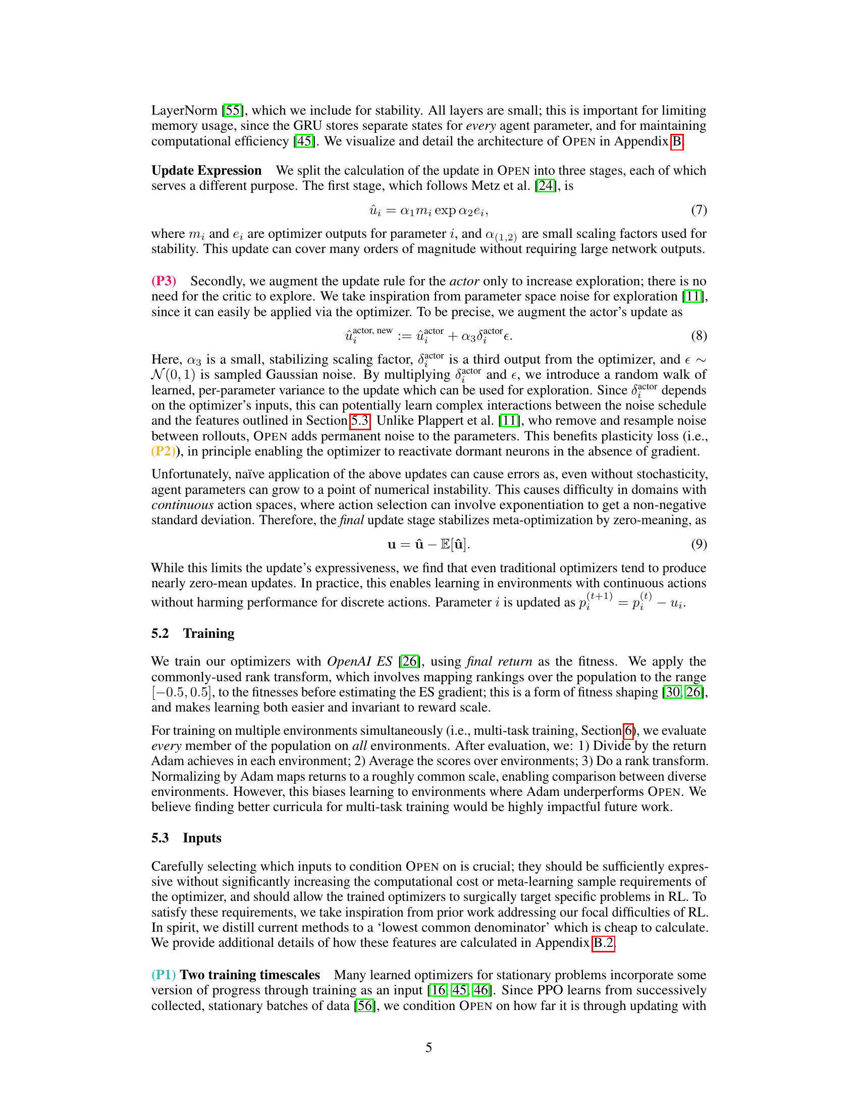
This figure presents the interquartile mean (IQM) of the final returns achieved by different optimizers (OPEN, No Features, Optim4RL, VeLO, Lion, RMSprop, Adam) across five single-task training environments (Freeway, Space Invaders, Breakout, Asterix, Ant). The results are averaged over 16 different random seeds for each environment, showing the robustness of the findings. 95% stratified bootstrap confidence intervals are also displayed to indicate the uncertainty in the measurements. The figure highlights the performance of OPEN relative to other optimizers, particularly in three of the five environments (Freeway, Asterix, Breakout), showcasing its strong performance in single-task training.

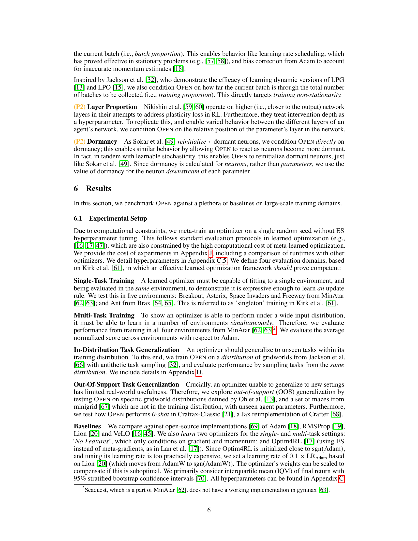
This figure compares the performance of different optimizers in a multi-task setting where they were trained on multiple environments simultaneously. The metrics shown are Mean, Interquartile Mean (IQM), and Optimality Gap. OPEN significantly outperforms all other optimizers across all three metrics, highlighting its ability to adapt to diverse learning environments.
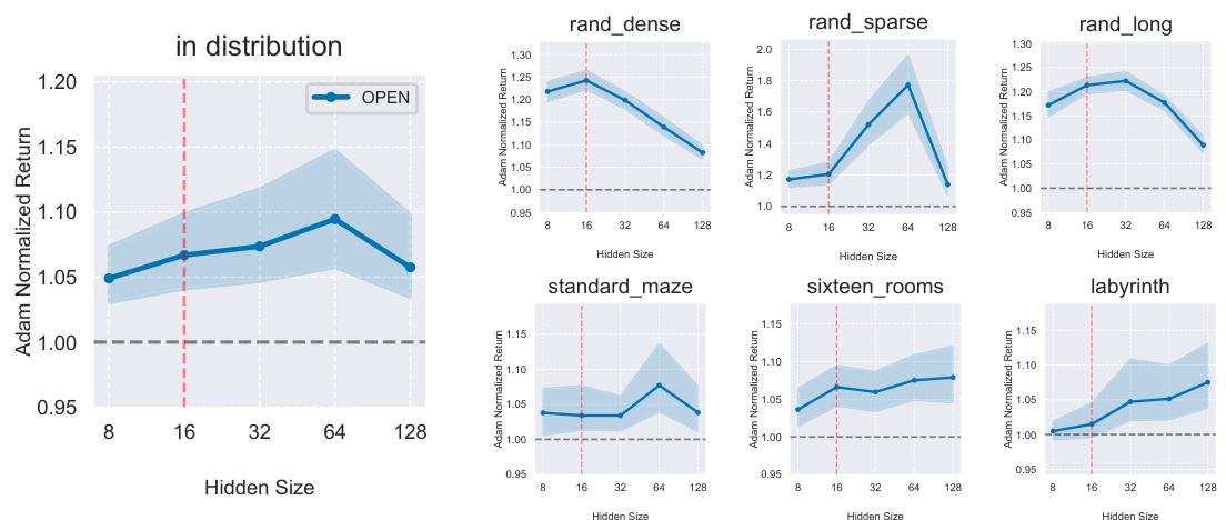
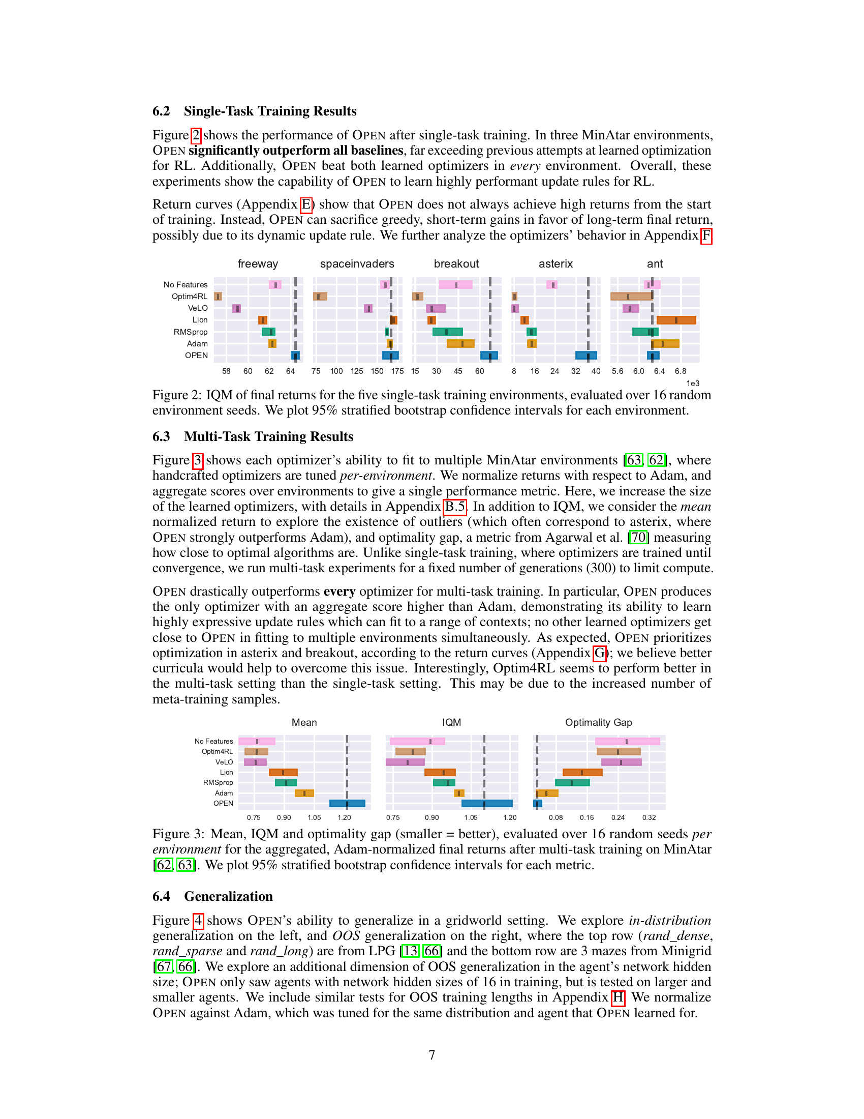
This figure shows the results of generalization experiments using the OPEN optimizer. The left panel shows results for gridworlds from the training distribution, demonstrating in-distribution generalization. The right panel shows out-of-distribution (OOS) generalization results on gridworlds and mazes from different distributions than those used in training. The results show OPEN’s ability to generalize to unseen tasks, both within and outside of the training distribution, and to different agent network sizes. The performance is normalized against Adam for comparison. Error bars represent 95% stratified bootstrap confidence intervals calculated across 64 random seeds.
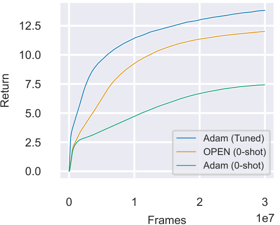
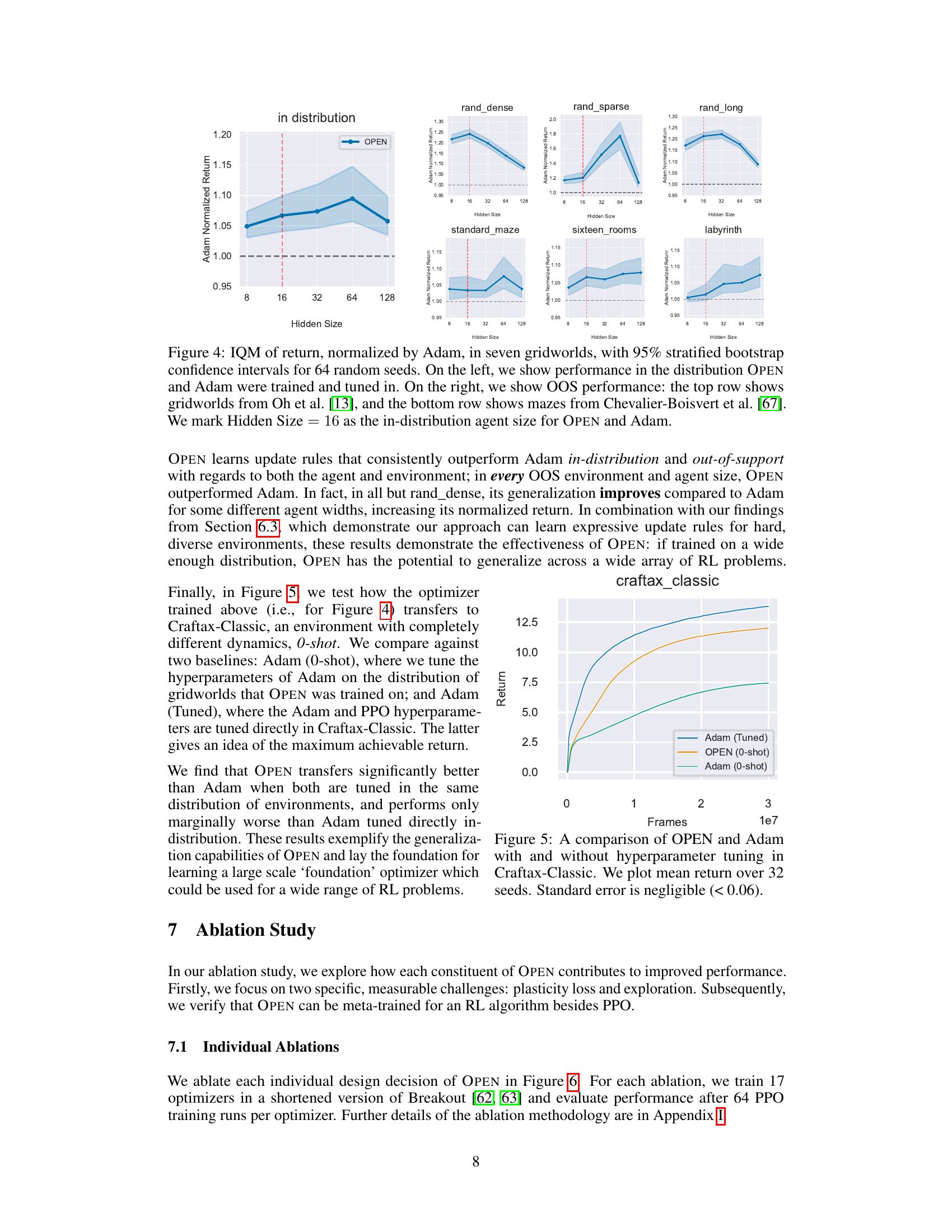
This figure compares the performance of OPEN and Adam in the Craftax-Classic environment, both with and without hyperparameter tuning. OPEN is evaluated in a zero-shot manner (i.e., without any prior training or tuning on Craftax-Classic), whereas Adam is tested both with and without tuning specifically for this environment. The results demonstrate OPEN’s ability to generalize effectively to a new environment, performing comparably to a finely-tuned Adam.

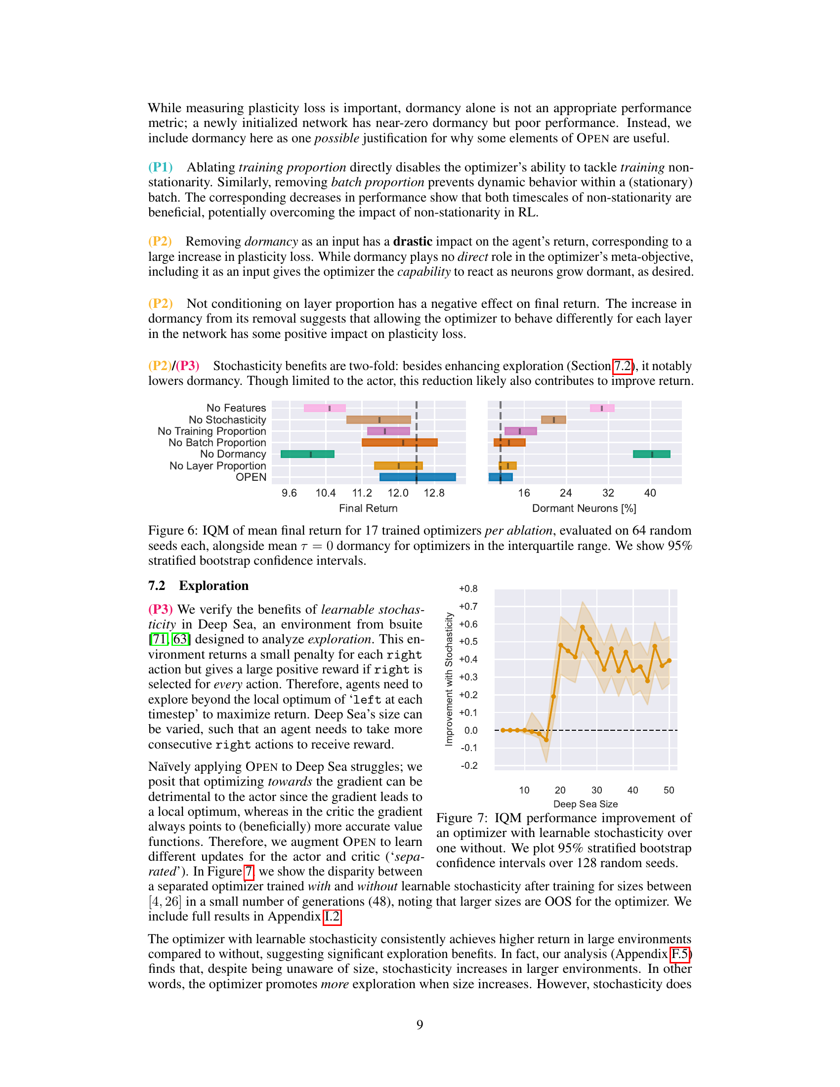
This figure shows the results of an ablation study on the OPEN algorithm. Seven different versions of the OPEN optimizer were created by removing one of its components (features or stochasticity). Each version was trained and tested on 64 random seeds, allowing the study to assess the effects of each component on performance. The results are summarized using the Interquartile Mean (IQM) of the final return for each optimizer, as well as the mean dormancy (proportion of inactive neurons). Error bars represent 95% stratified bootstrap confidence intervals. The figure clearly illustrates the importance of each component of the algorithm, demonstrating that the full OPEN optimizer achieves significantly better results than any of its ablated variants.
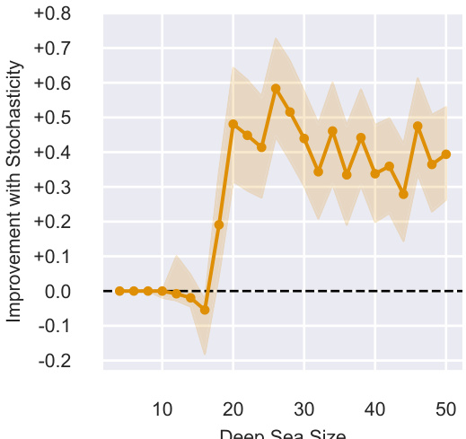
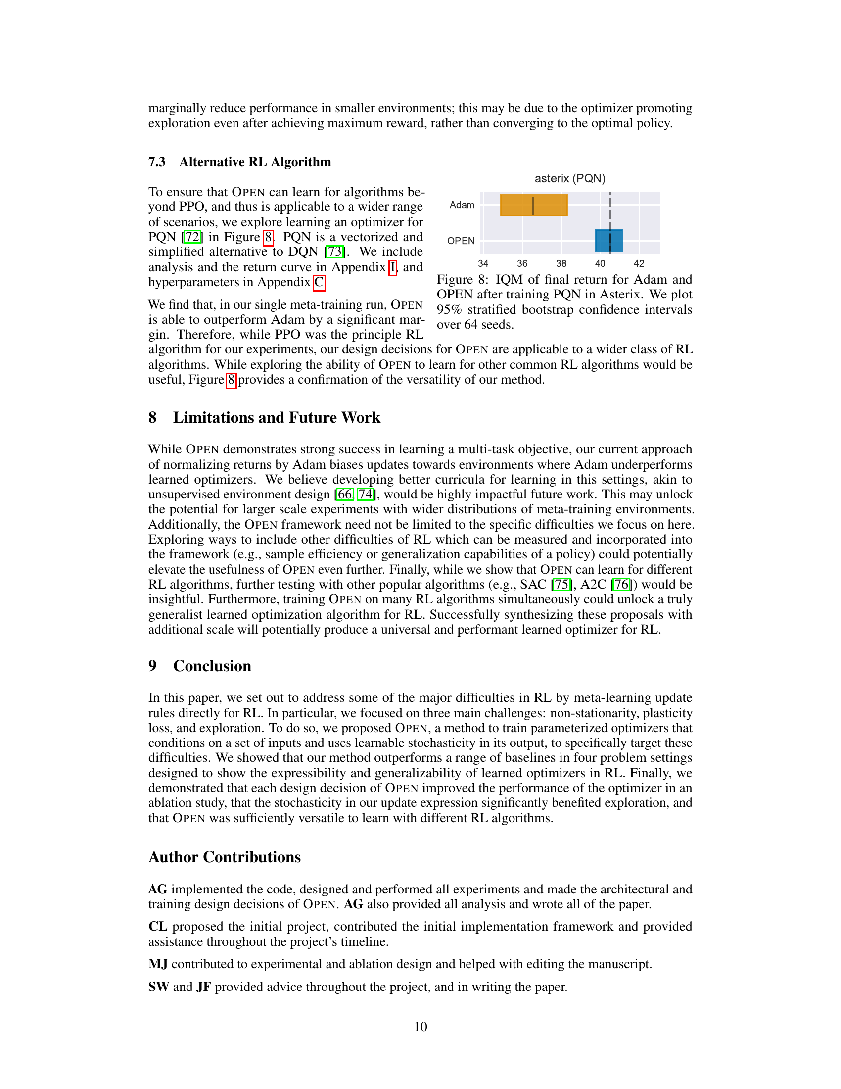
This figure shows the improvement in IQM (Interquartile Mean) performance when using an optimizer with learnable stochasticity compared to one without stochasticity. The experiment was conducted on the Deep Sea environment from the bsuite benchmark, varying the size of the environment (number of consecutive ‘right’ actions required to receive a reward). The results are shown for different environment sizes, with error bars representing 95% stratified bootstrap confidence intervals over 128 random seeds. The plot demonstrates the beneficial effect of learnable stochasticity, especially in larger environments, indicating its role in effective exploration.
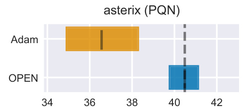
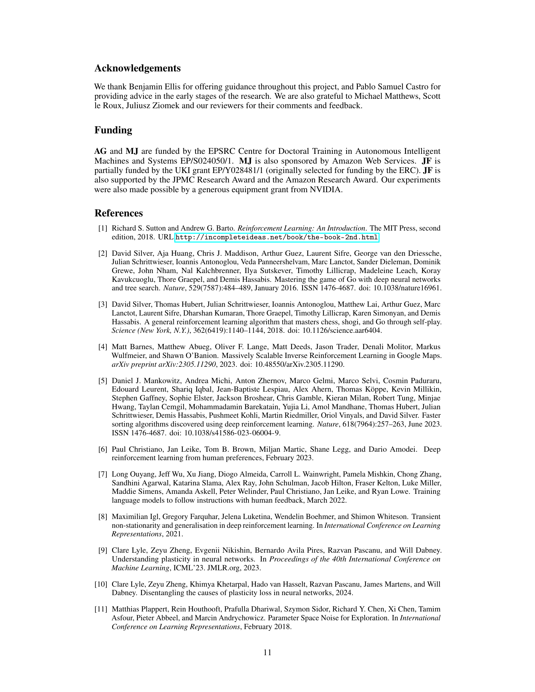
The figure shows the interquartile mean (IQM) of final returns for both Adam and OPEN optimizers when training a Proximal Q-Network (PQN) agent in the Asterix environment. The results are based on 64 random seeds, providing robust statistical estimates of performance. Error bars indicate 95% stratified bootstrap confidence intervals. This figure demonstrates that OPEN consistently outperforms Adam in this specific setting. It is a direct comparison evaluating how effectively each optimizer learns the update rules for the PQN algorithm, illustrating OPEN’s superior performance.

This figure illustrates the OPEN algorithm’s meta-learning process. Multiple RL agents are trained, each using a different optimizer sampled from a meta-learner. These optimizers receive gradient and momentum information, along with other context-specific features, to compute updates. The performance of each agent, measured by its final returns, is fed back into the meta-learner to refine the optimizer’s behavior over time. This iterative process allows the meta-learner to evolve better optimizers specifically tailored for the challenges of RL.

This figure shows the results of an ablation study on the Deep Sea environment. The study explores the impact of learned stochasticity and separate actor-critic parameters on the optimizer’s ability to generalize across different environment sizes. The results demonstrate that only the optimizer with both features is capable of generalization.
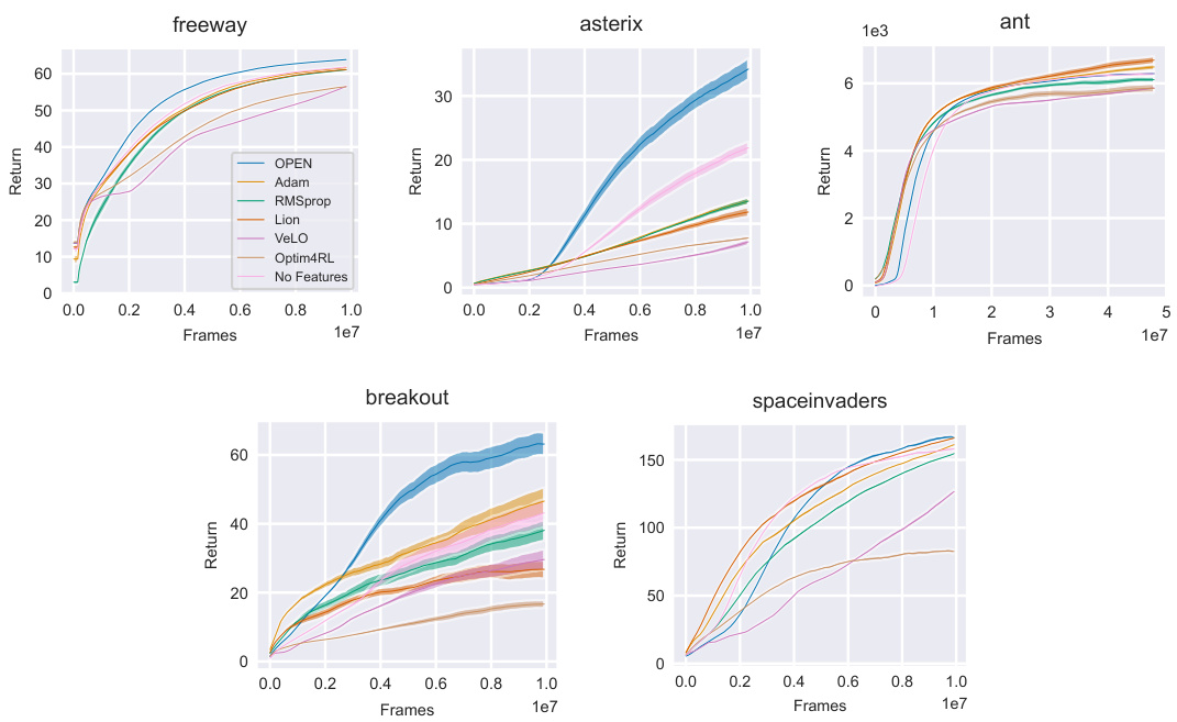
This figure compares the performance of different optimizers in reinforcement learning (RL) for five different single-task environments. The optimizers include OPEN (the proposed method), Adam, RMSprop, Lion, VeLO, Optim4RL, and No Features (a baseline). The curves show mean return with standard error over 16 random seeds, showcasing the progress of each optimizer over training time in each environment. The results demonstrate OPEN’s ability to learn highly performant update rules.

This figure displays the dormancy (a measure of neuron inactivity) over training time for different optimizers in four MinAtar environments. The plot shows the mean dormancy (with standard error bars) for each optimizer across 16 independent training runs. The purpose is to compare the plasticity (ability to retain activity in neurons) of different optimizers over the training process.
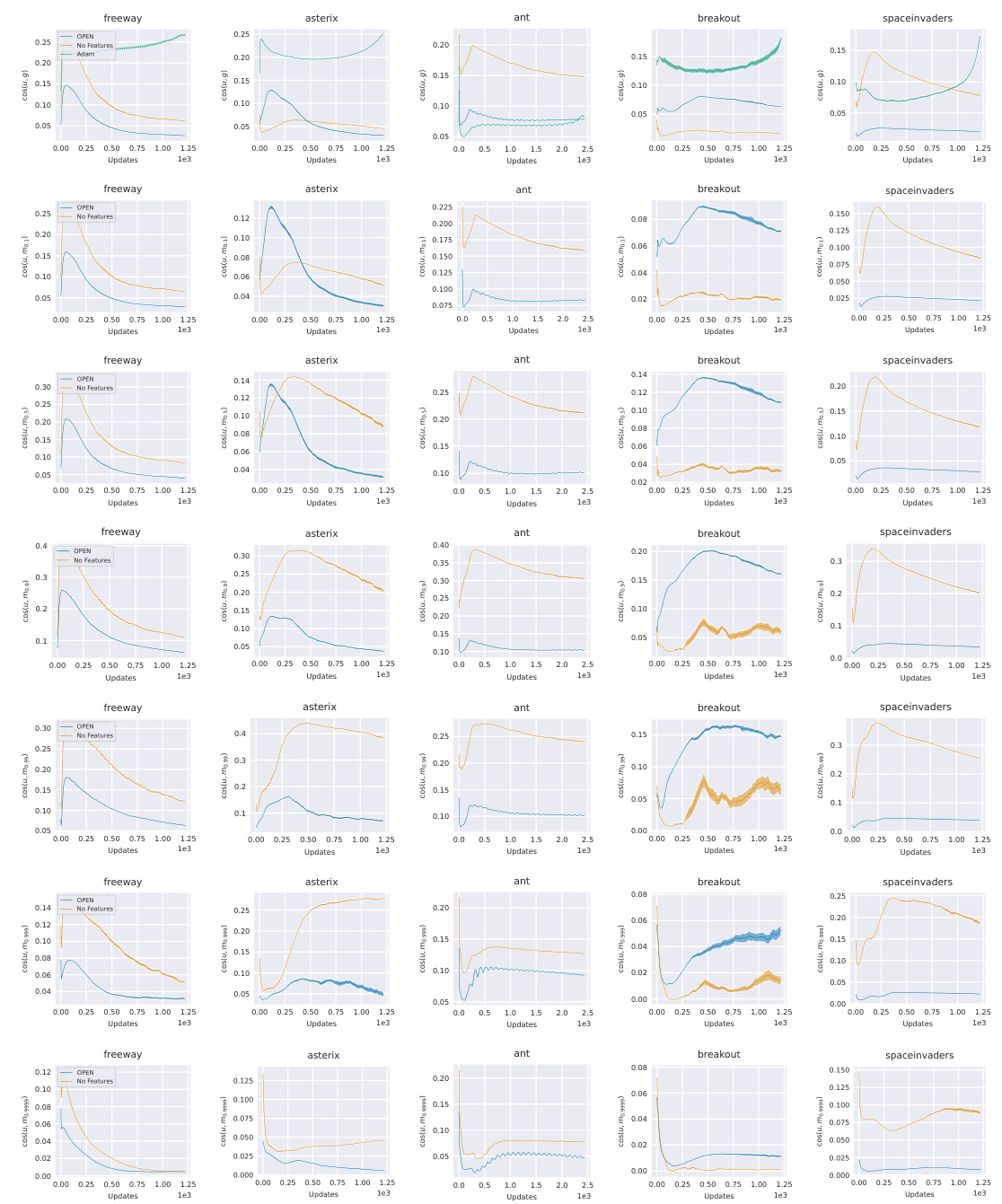
This figure shows the cosine similarity between updates generated by OPEN and a simpler optimizer (‘No Features’) against the gradient and momentum with different timescales (β values). The results are presented for each of the five MinAtar environments. The figure aims to illustrate the relationship between OPEN’s updates and traditional optimization components like gradient and momentum across various timescales.

This figure shows the cosine similarity between updates generated by OPEN and a baseline method (‘No Features’) against the gradient and momentum at different timescales. The analysis helps to understand how OPEN’s updates relate to standard optimization methods (gradient and momentum) across various environments and timescales. The use of different beta values (β) for momentum calculation allows the examination of these relationships at various levels of smoothing.

This figure shows the cosine similarity between updates generated by OPEN and a simpler model, ‘No Features’, against gradients and momentum with different beta values. The analysis shows that both optimizers align with momentum at similar timescales to those tuned in Adam, while the additional elements of OPEN cause less similarity to ‘No Features’.

This figure visualizes how the weight of the learned stochasticity (factor) changes over time during training. The stochasticity is incorporated into the actor’s update rule as follows: ûactor = ûactor + α3δactorε, where ε is sampled from a standard normal distribution N(0,1). The y-axis shows the normalized stochasticity weight (randomness/p), calculated as |ûactorε|/p, where p is the parameter value. The x-axis represents the number of updates. The plot includes separate lines for five different environments (freeway, asterix, ant, breakout, spaceinvaders), each showing the mean normalized stochasticity weight with standard error calculated across 16 random seeds. The plot shows that the stochasticity weight generally decreases over time, suggesting that the model prioritizes exploration early in training and exploitation later, which is expected.
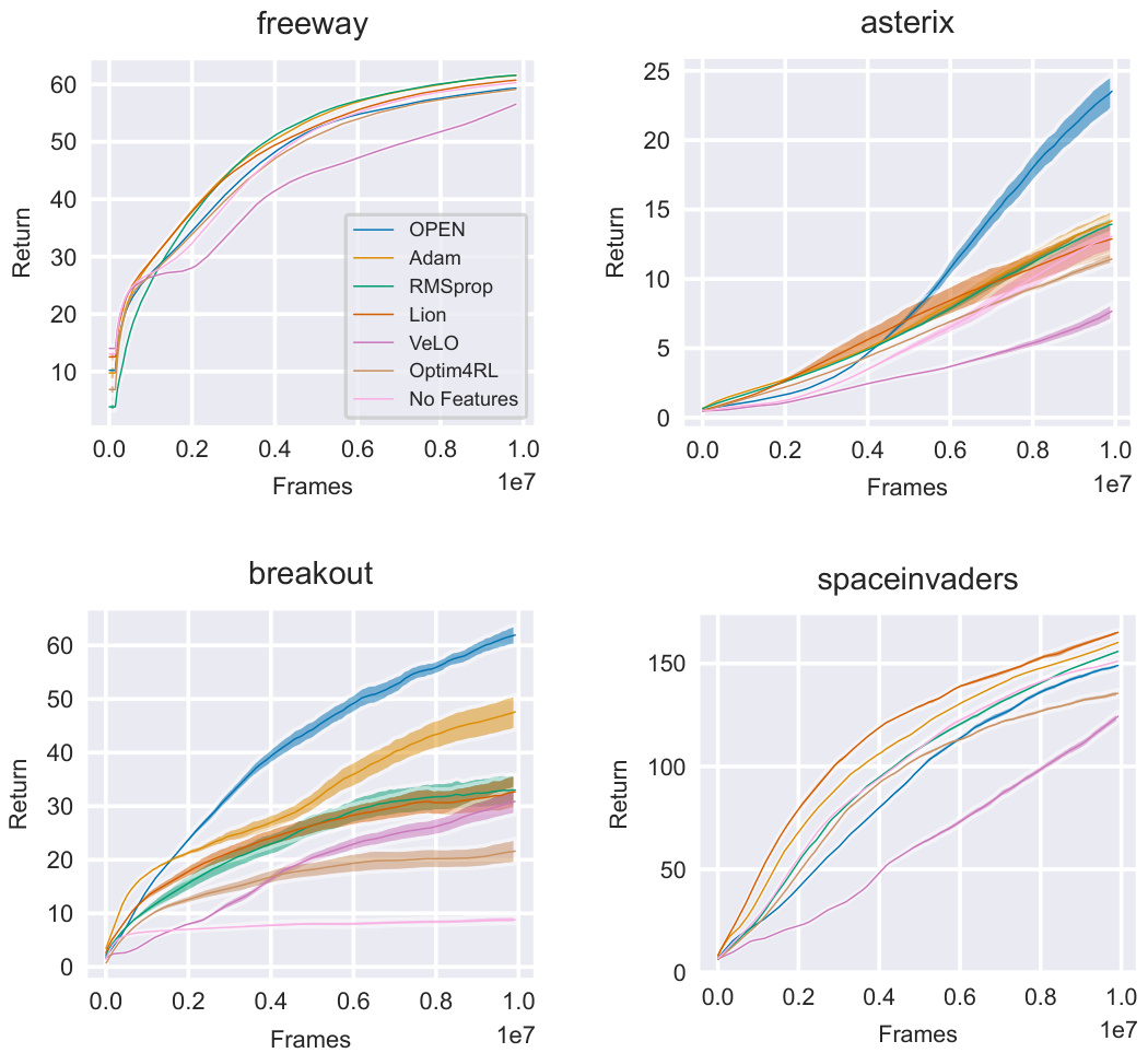
This figure compares the performance of different optimizers in reinforcement learning (RL) during training on five different single-task environments (Freeway, Asterix, Breakout, SpaceInvaders, Ant). The curves show the average return obtained by each algorithm over many training iterations (frames). The results illustrate the learning speed and final performance of the proposed Learned Optimization for Plasticity, Exploration, and Non-stationarity (OPEN) method compared to traditional optimizers such as Adam and RMSprop, and other learned optimizers.

This figure demonstrates the generalization capabilities of OPEN across different gridworld environments. The left side shows results for environments within the training distribution, highlighting OPEN’s consistent outperformance of Adam. The right side assesses out-of-distribution generalization, revealing that OPEN maintains superior performance across varied gridworld types and agent network sizes. This underscores OPEN’s ability to adapt and generalize beyond its training data.
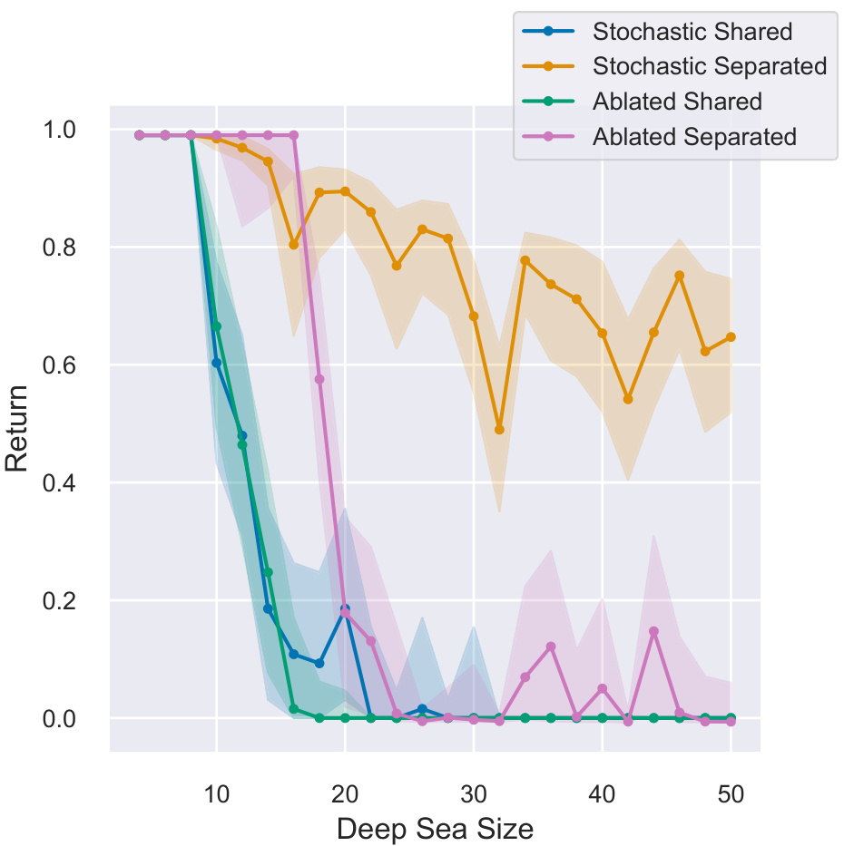
This figure shows the results of an ablation study on the Deep Sea environment, which tests the ability of different optimizers to generalize to different problem sizes. The results show that the optimizer with separate parameters for the actor and critic, and with learned stochasticity, is the only one that generalizes well across a wide range of problem sizes. The other optimizers either perform poorly in larger environments or do not generalize at all.

This figure shows the training curves for the PQN algorithm in the Asterix environment, comparing the performance of OPEN and Adam as optimizers. The x-axis represents the number of frames (training steps), and the y-axis represents the mean return achieved by each optimizer. Error bars indicate standard error calculated over 64 independent runs. The plot illustrates that OPEN initially achieves lower returns than Adam at the beginning of training but eventually surpasses Adam’s performance in the later stages.
More on tables
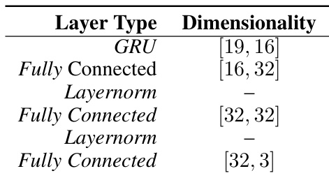
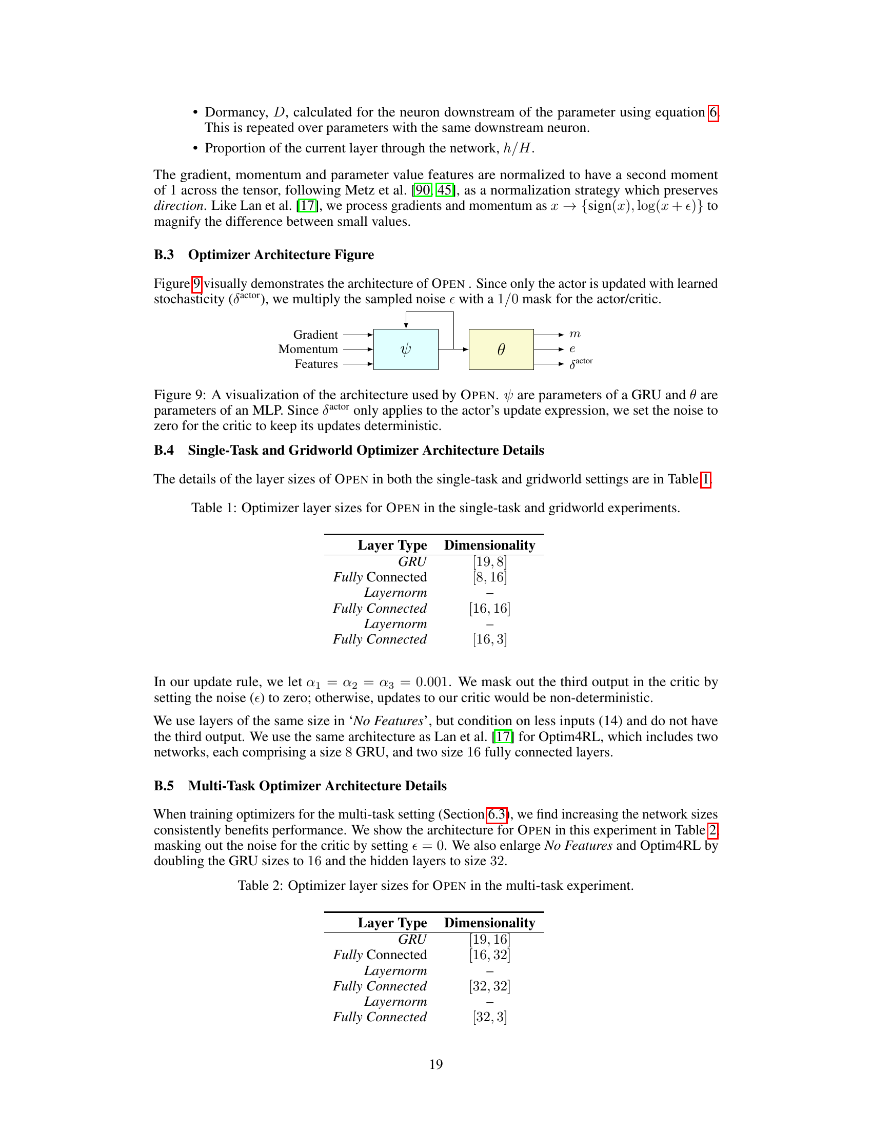
This table presents the architecture of the optimizer used in the multi-task experiment. It shows the different layers used in the optimizer, including GRU (Gated Recurrent Unit), fully connected layers, and LayerNorm layers. The dimensionality of each layer is also specified. The architecture is designed to handle the complexities of multi-task learning by conditioning on multiple inputs and using a gated recurrent unit for capturing temporal dependencies. The use of small layer sizes is a design choice to limit memory usage and maintain computational efficiency.
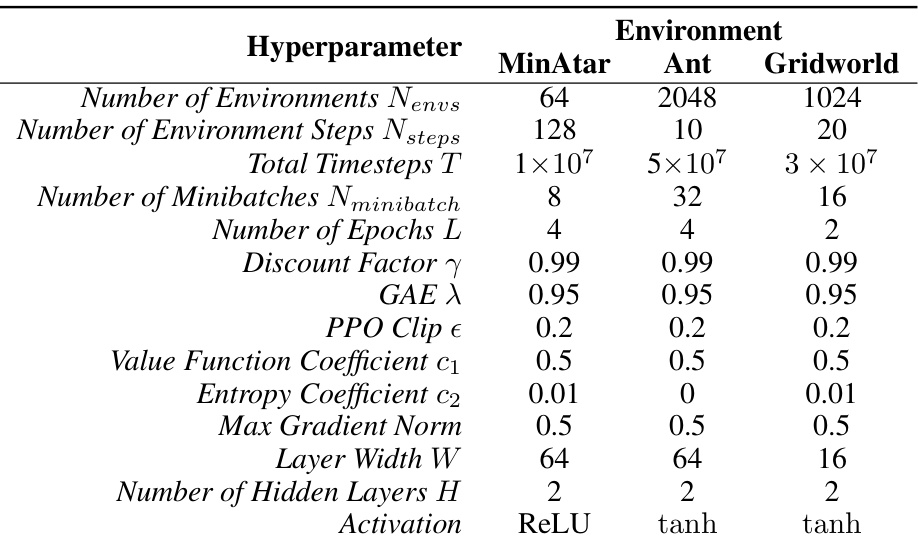
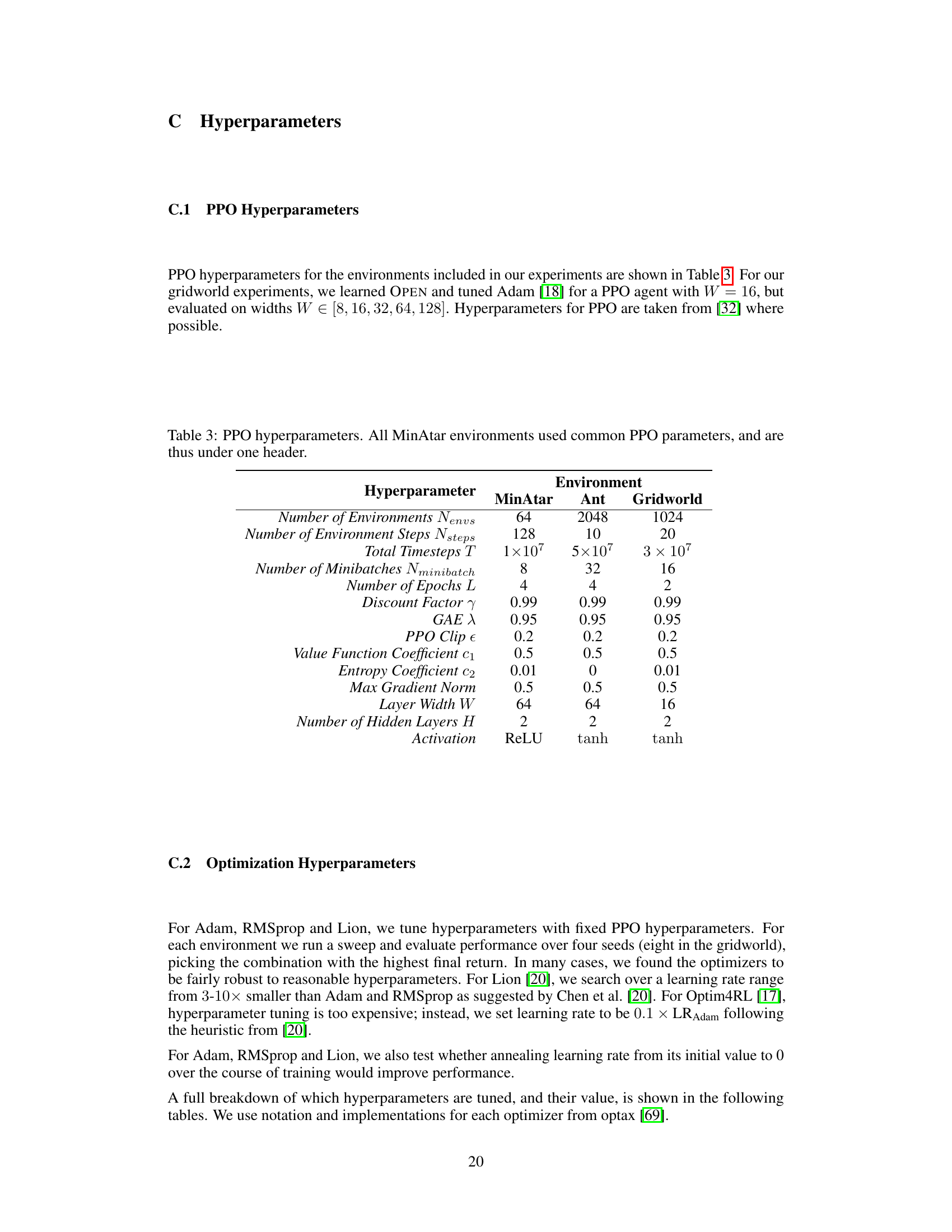
This table lists the hyperparameters used for the Proximal Policy Optimization (PPO) algorithm in the experiments described in the paper. It shows the settings used across different environments (MinAtar, Ant, Gridworld). The hyperparameters control various aspects of the PPO algorithm, such as the number of training steps, batch sizes, learning rates, and other parameters that affect the training process. The consistency in hyperparameters across MinAtar environments highlights the authors’ focus on controlling variables to isolate the effects of the optimization algorithm itself.
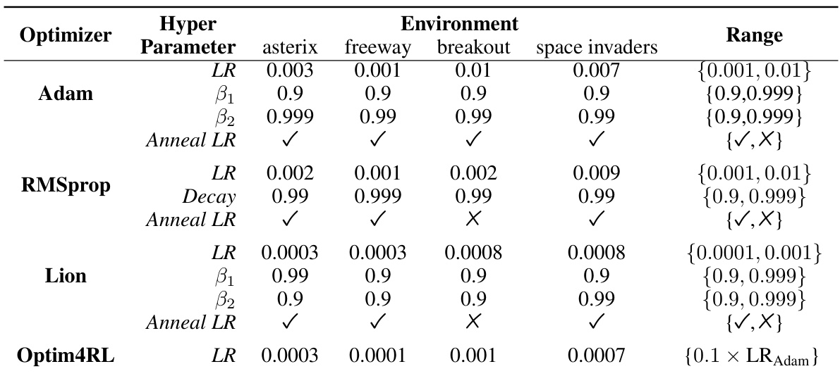
This table presents the hyperparameters used for Adam, RMSprop, Lion, and Optim4RL optimizers in the MinAtar environment. For each optimizer, it shows the learning rate (LR), beta1 (β1), beta2 (β2), decay (RMSprop only), and whether learning rate annealing was used. The ‘Range’ column specifies the range of values explored during hyperparameter tuning for each parameter. The table details the values used for each environment (asterix, freeway, breakout, space invaders) during hyperparameter tuning, highlighting the different configurations explored for each algorithm.
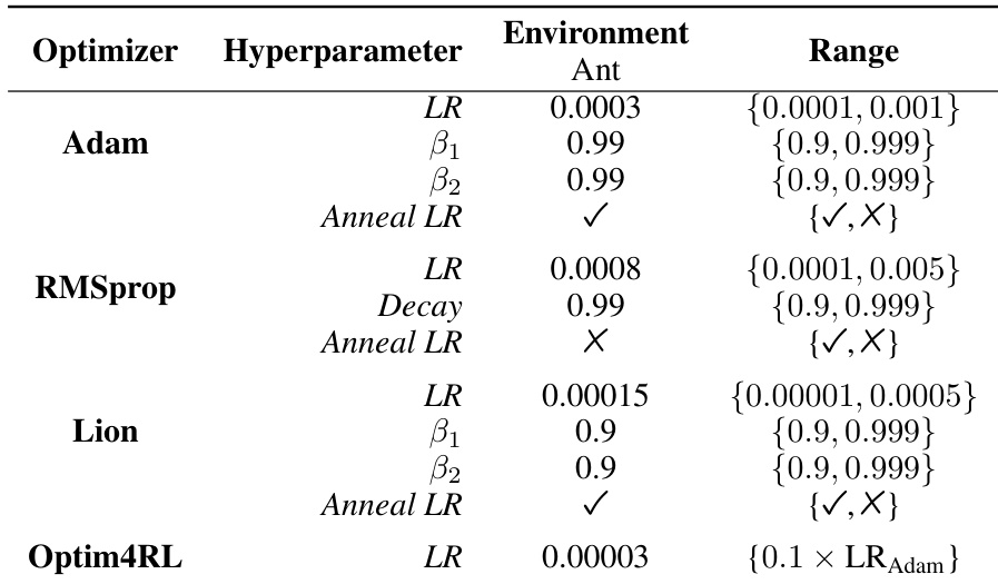
This table presents the hyperparameters used for the Adam, RMSprop, Lion, and Optim4RL optimizers when applied to the Ant environment. For each optimizer, it lists the learning rate (LR), beta1 and beta2 parameters (for Adam, RMSprop, and Lion), the decay parameter (for RMSprop), and whether learning rate annealing was used (Anneal LR). The ‘Range’ column specifies the range of values explored during hyperparameter tuning for each optimizer in the Ant environment.

This table shows the hyperparameters used for the Adam optimizer when training on the gridworld environment. It lists the hyperparameters (learning rate (LR), beta1, beta2) and whether learning rate annealing was used. The ‘Range’ column indicates the range of values tested during hyperparameter tuning to find the optimal settings for each of these parameters.
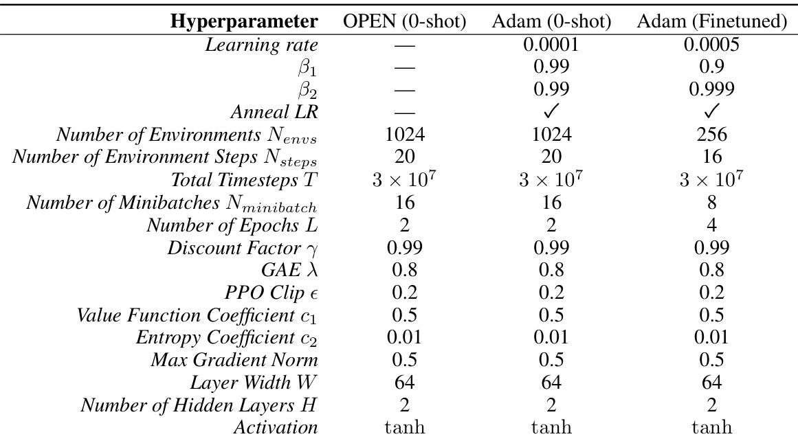
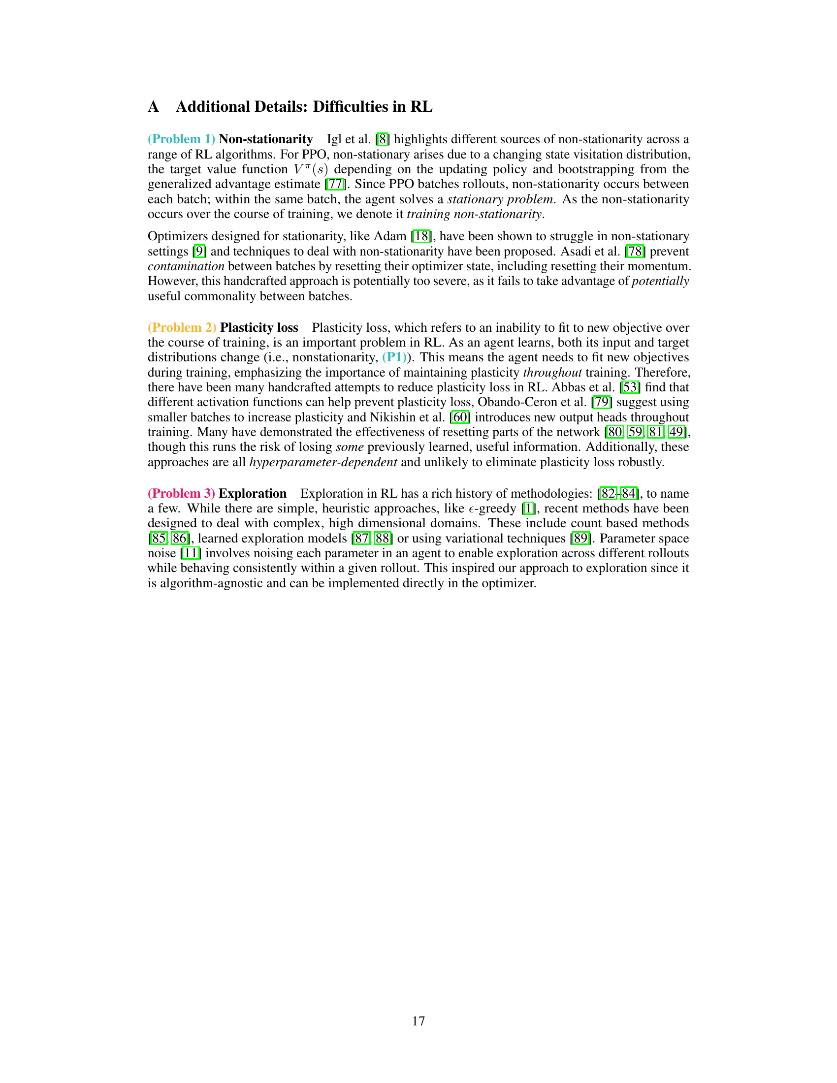
This table presents the hyperparameters used for training the PPO agent in the Craftax-Classic environment. It compares the hyperparameters used for the OPEN optimizer (0-shot), Adam optimizer (0-shot), and Adam optimizer (finetuned). The table includes parameters such as the learning rate, beta1, beta2, whether or not learning rate annealing was used, the number of environments, environment steps, total timesteps, number of minibatches, number of epochs, discount factor, GAE lambda, PPO clip epsilon, value function coefficient, entropy coefficient, max gradient norm, layer width, number of hidden layers, and activation function.
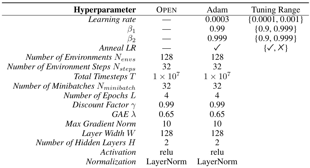
This table shows the hyperparameters used for the Proximal Policy Optimization (PPO) algorithm in the experiments. It lists hyperparameters such as the number of environments, number of environment steps, total timesteps, number of minibatches, number of epochs, discount factor, GAE lambda, PPO clip epsilon, value function coefficient, entropy coefficient, max gradient norm, layer width, number of hidden layers and activation function. Note that the MinAtar environments all used the same PPO hyperparameters, hence they are grouped under a single header.
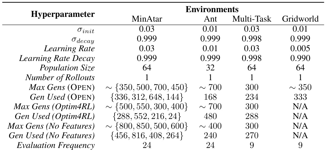
This table presents the hyperparameters used for training the optimizers with ES. It shows the initial standard deviation (σinit), decay rate (σdecay), learning rate, learning rate decay, population size, number of rollouts, maximum number of generations, generation used for evaluation, and evaluation frequency for the different environments (MinAtar, Ant, Multi-Task, Gridworld). The values reflect choices made to balance computational cost and performance, notably with differing maximum generation numbers for different optimizers and environments.
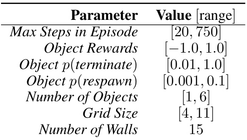
This table lists the parameters used to generate the gridworld environments for training the OPEN optimizer. It shows the ranges from which the values for each parameter are randomly sampled during training. This randomization helps the optimizer generalize to a wider variety of gridworld environments. Each parameter represents a characteristic of the gridworld environment such as the maximum number of steps in an episode, the range of rewards received from objects, and the probability of those objects terminating or reappearing. The number of walls and the size of the grid are also specified.
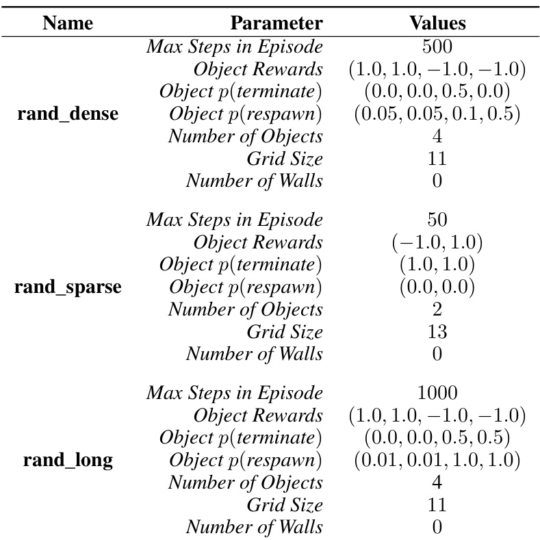
This table presents the parameters used to generate the gridworld environments for testing OPEN’s generalization capabilities. It lists the specific values used for three different gridworld configurations:
rand_dense,rand_sparse, andrand_long. For each configuration, the table details the maximum steps allowed in an episode, the rewards associated with each object, the probabilities of object termination and respawning, the number of objects, the size of the grid, and the number of walls present. These parameters control the complexity and characteristics of the gridworld environments, allowing for a systematic evaluation of the algorithm’s ability to generalize to unseen environments.
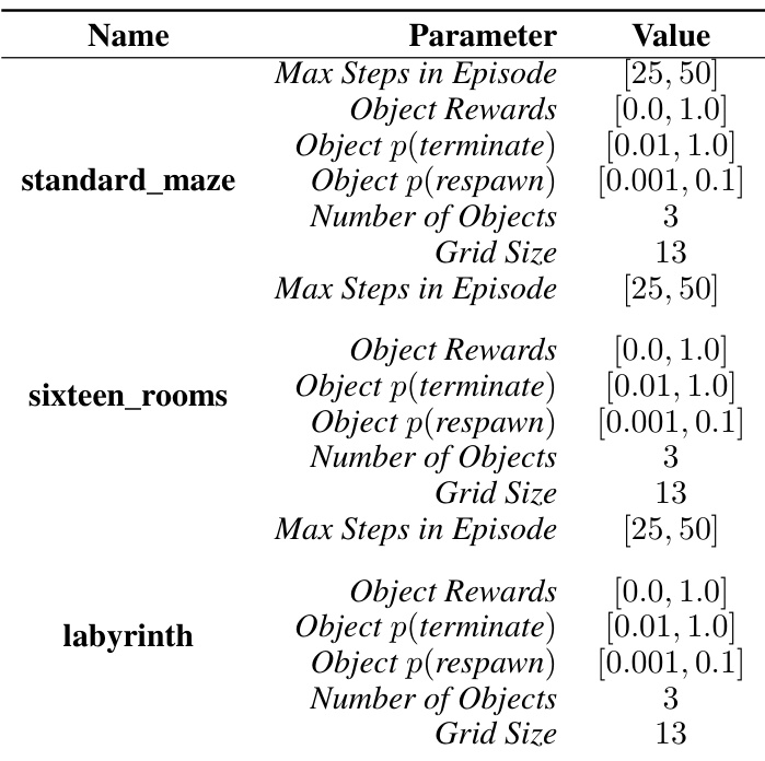
This table lists the parameters used to generate gridworld environments for testing. The ‘Name’ column specifies the type of gridworld (standard_maze, sixteen_rooms, labyrinth). Each row then details the range of values sampled for each parameter (Max Steps in Episode, Object Rewards, Object p(terminate), Object p(respawn), Number of Objects, Grid Size) during testing. The ranges ensure variability across different test runs.
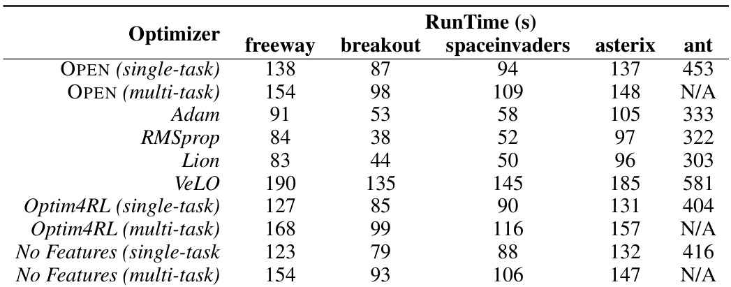
This table shows the inference time in seconds for different optimizers across five different environments. The experiments were run on four L40s GPUs, leveraging Jax’s parallel processing capabilities. The table allows for a comparison of the computational efficiency of different optimizers, highlighting the trade-off between speed and performance.
This table shows the layer sizes and dimensionality of the different layers in the OPEN optimizer for single-task and gridworld experiments. It breaks down the architecture of the optimizer, specifying the type of layer (GRU, Fully Connected, Layernorm), and its dimensionality (number of nodes). This is important for understanding the model’s capacity and complexity.
Full paper#
